Open Science Repository Mathematics

doi: 10.7392/Mathematics.70081944

Lyapunov’s Second Method for Estimating Region of Asymptotic Stability

Zelalem Yadeta

Haramaya University

Abstract

This seminar basically consists of three chapters. The first chapter converses the background about Lyapunov’s second method of estimating region of asymptotical stability (RAS) and mathematical preliminaries which will be needed in the next two chapters. The second chapter deals with Lyapunov’s second method for estimating region of asymptotic stability of autonomous nonlinear differential system. Chapter three deals with estimating region of asymptotic stability of nonautonomous system. Finally I summarize Lyapunov’s second method of estimating RAS.

Keywords: Lyapunov’s second method, asymptotic stability, autonomous nonlinear differential system, nonautonomous system.

1. Introduction

1.1 Background

The subject of this analysis is to estimate region of asymptotic stability using Lyapunov’s second method in differential equations (nonlinear dynamic system). This technique was discovered by Lyapunov’s in the 19^th century. The technique is also called direct method because this method allows us to determine the stability and asymptotic stability of a system without explicitly integrating the nonlinear differential equation.

Lyapunov’s second method also determines the criteria for stability and asymptotical stability. In addition to giving us these criteria, it gives us the way of estimating region of asymptotic stability. Asymptotic stability is one of the stone areas of the qualitative theory of dynamical systems and is of fundamental importance in many applications of the theory in almost all fields where dynamical effects play a great role.

In the analysis of region of asymptotic stability properties of invariant objects, it is very often useful to employ what is now called Lyapunov’s second method. It is an important method to determine region of asymptotic stability. This method relies on the observation that asymptotic stability is very well linked to the existence of a Lyapunov’s function, that is, a proper, nonnegative function, vanishing only on an invariant region and decreasing along those trajectories of the system not evolving in the invariant region. Lyapunov proved that the existence of a Lyapunov’s function guarantees asymptotic stability and, for linear time-invariant systems, also showed the converse statement that asymptotic stability implies the existence of a Lyapunov’s function in the region of stability.

Converse theorems are interesting because they show the universality of Lyapunov’s second method. If an invariant object is asymptotically stable then there exists a Lyapunov’s function. Thus there is always the possibility that we may actually find it, though this may be hard.

When we mention Lyapunov’s second method to estimate region of stability, particularly for asymptotical stability, we have to know first the properties of asymptotical stability of



dynamic system at equilibrium point = 0 at if the following two conditions are satisfied

1) x* = 0 is stable, and
2) x* = 0 is locally attractive; i.e., there exists such that < δ


1.2 Objectives

The main objective of this seminar is to estimate region of asymptotical stability of nonlinear differential equation for both autonomous and nonautonomous systems using Lyapunov’s second method. This directly influences the exact estimating region of the asymptotic stability.

Hence this seminar is deliberately to explore the following specific objectives:

• To provide the methods for determining region of asymptotical stability (RAS)
• To analyze and demonstrate region of asymptotic stability basically using Lyapunov’s second method.
• To analyze some related theorem, application and examples of region of asymptotical stability.


1.3. Mathematical preliminaries

In this subtopic we deal with some mathematical results which will be needed later and we state some general principles related to Lyapunov’s second method to estimating region of asymptotic stability


1.3.1 Lyapunov’s functions

Lyapunov’s functions are a powerful function for determining the stability or instability of fixed points of nonlinear autonomous systems. To explain the method, we begin with a few definitions. We study an autonomous system

(1.1)

We assume that x and f(x) are in. The domain of f may be an open subset of, but we will only be interested in what happens near a particular point, so we won't complicate the notation by explicitly describing the domain of f.

Let V be a real valued function defined on an open subset U of and let p be a point in U. We say that V is positive definite with respect to p (or just positive definite, if p is understood) if for all x U and V (x) = 0 if and only if x = p.

Suppose that V in . We want to examine the derivative of V along trajectories of the
system Suppose that is a solution of Then, we have

(1.2)

where denotes the usual dot product inand

,

is the gradient vector of V. Since x is a solution of (1.1) we may rewrite (1.2)



Thus, if we define a function we have .

It is trivial, but important, to observe that we can compute without having to solve the system explicitly. Where V(x) is Lyapunov’s functions


1.3.2 Stability in the sense of Lyapunov’s second method

Let (1.3) be dynamic system that satisfies all the standard condition existence and uniqueness of solutions. A point is equilibrium point of the system, if .


Definition: The equilibrium point x* = 0 (assume x* is isolated critical point) of equation (1.3) is stable (in the sense of Lyapunov’s) at if for any there existssuch that < δ . Lyapunov’s stability is a very gentle requirement on equilibrium points. In particular, it does not require that trajectories starting close to the origin tend to the origin asymptotically. Also, stability is defined at a time instant. Uniform stability is a concept which assures that the equilibrium point is not losing stability. We state that for a uniformly stable equilibrium point, δ in the definition of stability in the sense of Lyapunov’s not be a function of , so that equation

< δ (1.4)

may hold for all.

Asymptotic stability is made precise in the following definition. In many physical situations, the origin may not be asymptotic stable for all possible initial conditions but only for initial conditions contained in region around the origin, such a region is called the region of asymptotic stability or finite region of attraction. If such region exists, computation of such a region is of great interest to the system designer.


Definition: An equilibrium point x* = 0 of (1) is asymptotically stable at if

x* = 0 is stable, and
x* = 0 is locally attractive; i.e., there exists such that

< δ (1.5)

As in the previous definition, asymptotic stability is defined at t₀.

Uniform asymptotic stability requires:

x* = 0 is uniformly stable, and
x* = 0 is uniformly locally attractive; i.e., there exists δ independent of t₀ for which equation (1.5) holds. Further, it is required that the convergence in equation (1.5) is uniform. In other words, a solution is called asymptotic stable if it is stable and attractive. Finally, we say that an equilibrium point is unstable if it is not stable.

In another way, the region of asymptotic stability of the origin is defined as the set of all points X₀ that and .

So, we can find an open invariant set Ω with boundary such that Ω is the region of asymptotic stability (RAS) of system (1.1) defined by the property that every trajectory starting from reaches the equilibrium point of the corresponding system.

a) Stable in the sense of Lyapunov b) Asymptotically stable

Figure 1.1: Phase portraits for stable and asymptotically stable.


Definition: A set A of points in E_n is (positive) invariant with respect to the system (1.1), if every solution of (1.1) starting in A remains in A for all future of time.


1.3.3 Basic theorem of Lyapunov’s

To state Lyapunov’s second method of estimating region of asymptotic stability first define the two definitions concerned with the construction of certain scalar function. Let V(x) be scalar continuous function, i.e. real-valued function of the variables defined on the region containing the origin again Ω could be the whole space.


Definition 1: The scalar function V(x) is said to be positive definite on the set if
V(0) =0 and V(x)>0 for and x in.


Definition 2: The scalar function V(x) is negative definite on the set if and only if -V(x) is positive definite on.


Example: If n=3 the function is positive definite, since V(y)>0 and V(0) (on the whole space), but the function , while obviously nonnegative, is not positive definite because v(0)=0 on the plane y₁=0 i.e. at every point of the (y_2,y₃) plane.


Definition: The derivative of V with respect to the system is the scalar product

(1.6)

Note that V*(x) can be computed directly from the differential equation without any knowledge of the solutions. Herein lies the power of Lyapunov’s method. We observe that if is any solution of (1.1), by rule the definition of solution, and (1.6) we have

(1.7)

In other words, along a solution the total derivative of V() with respect to t coincides with the derivatives of V with respect to the system evaluated at x=.


Example 2: For the system

and the given function

We obtain, using the definition (1.6) with



With these definitions, we may state the basic theorem as follows.


Theorem 1: Let p be a fixed point of the system



Let U be an open neighborhood of p and let be a continuous function that is positive definite with respect to p and is C¹ on U, except possibly at p. Then, the following conclusions can be drawn:

a. If on, then p is a stable fixed point for
b. If on, then p is an asymptotically stable fixed point for

Geometrically, the condition says that the vector field f points inward along level curves of V. If V is positive definite with respect to p, it seems reasonable that level curves of V should enclose and close in U on p, so p should be stable.

A function satisfying the conditions in the theorem and (a) is called a Lyapunov’s function for f at p. If it satisfies (b), it is called a strict Lyapunov’s function.


Proof: Let and be given. Assume, without loss of generality, thatis contained in D. Assume positive definite function W: such that V (t; x) W(x) for every (t; x) R D. Let m = min Since W is continuous and positive definite, m is well-defined and positive. Given that > 0 small enough that < and max{}.

Since V is positive definite and continuous function, it is possible to, if x(t) solution

of and then, and
for all t, so V (t; x(t)) < m for every t t0. Thus, W(x(t)) < m for every t t₀, so, for every t t₀, . Since, this tells us that

for every t t₀. The solution of is stable.


Example 1: Mass on spring.

Consider a point mass with mass m attached to a spring, with the mass constrained to move along a line. Let y denote the position of the mass, with y = 0 the equilibrium position. Moving the mass in the positive y direction stretches the spring and moving the mass in the negative y direction compresses the spring. According to Hooke's law, the force exerted by the spring is

F = -ky,

for some constant k > 0 (this is an approximation that is good for displacements that are not to large).

Applying Newton's law F = ma, we see that the differential equation governing the motion of the mass is:

Appropriate initial conditions are the initial position and velocity of the mass. Of course, we can solve this equation explicitly to show that all of the motions are periodic and the equilibrium position (y = 0, velocity = 0) is stable. But, for illustration, let's prove that the equilibrium is stable using a Lyapunov function.

There is an obvious choice from physics, the total energy of the system.

The work done against the spring in moving from 0 to y is



This is the potential energy of the system at position y. The kinetic energy is , where v is velocity.

The total energy is



To apply Lyapunov's theorem, we need to convert the second order equation to a first order system. Using x₁ = y, x₂ = = v, the result is



Thus, the equation is where



Looking at our expression for the energy, we take



This is clearly positive definite with respect to the origin. The gradient of V is



Thus, we have , this means energy is conserved.

This shows that the origin is stable.


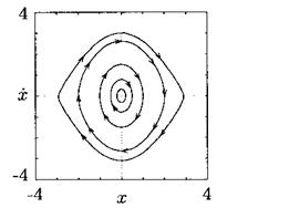
Example 2: Consider the planar system

(i)

The origin is a fixed point. Take , which is clearly positive definite with respect to the origin. Rather than computing , we can do the same computation by differentiating V (x, y), assuming that x and y are solutions of (i). Thus, we have



Thus, on, so 0 is an asymptotically stable fixed point for the system (i).

See figure below for a picture of the phase portrait of this system near the origin.

Figure 1.2: The origin is asymptotically stable for the system of (i) (texas.math.ttu.edu)


Definition: A continuous function V: Rⁿ × R+ → R is decrescent if for some and some continuous, strictly increasing function β : R₊ → R,

.


Theorem 2: Let V (x, t) be a non-negative function with derivative along the trajectories of the system.

1. If V (x, t) is locally positive definite and locally in x and for all t, then the origin of the system is locally stable (in the sense of Lyapunov’s).
2. If V (x, t) is locally positive definite and decrescent, and locally in x and for all t, then the origin of the system is uniformly locally stable (in the sense of Lyapunov’s).
3. If V (x, t) is locally positive definite and decrescent, and is locally positive definite, then the origin of the system is uniformly locally asymptotically stable.
4. If V (x, t) is positive definite and decrescent, and is positive definite, then the origin of the system is globaly uniformly asymptotically stable.

Since the theorem 2 only gives sufficient conditions, the search for a Lyapunov’s function establishing stability of an equilibrium point could be arduous. However, it is a remarkable fact that the converse of this theorem also exists. If an equilibrium point is stable, then there exists a function V (x, t) satisfying the conditions of the theorem. However, the utility of this and other converse theorems is limited by the lack of a computable technique for generating Lyapunov’s function.

We present a converse Lyapunov’s result for nonlinear time-varying systems that are uniformly semi globally asymptotically stable. This stability property pertains to the case when the size of initial conditions may be arbitrarily enlarged and the solutions of the system converge, in a stable way, to a closed ball that may be arbitrarily diminished by change a design parameter of the system (typically but not exclusively, a control gain). This result is notably useful in cascaded-based control when uniform practical asymptotic stability is established without a Lyapunov’s function. We provide a tangible example by solving the stabilization problem of a hovercraft.


Theorem: If there exists a scalar function V(x) that is positive definite and for which V*(x) is negative definite on some region Ω containing the origin, then the zero solution of (1.1) is asymptotically stable.


Proof: If there is a solution stable in Ω, there exist sphere radius contained in the region Ω center at origin of the phase plane, such that and . In particular, for, there exists such that all solution of (*) with and exist on and satisfy ().

We have a non-increasing function V() of t which is bounded below. Therefore exists. Suppose that for some we could have

for (**)

We will show that (**) is impossible. By continuity, for the , there exists a 0< such that whenever ||x||< (***)
.
Therefore, the solution for which (**) holds must satisfy |||| for t Let S be the set of y lying between the spheres of radius and r, that is, S={x|}. Consider the function -V*(x) on the closed bounded set S. By hypothesis on f and V, -V*(y) define (1.6) is continuous and positive definite.

Let



Since 0 is not a point of S we have using also (1.7)

()

Integrating, we obtain V( for . But then clearly for t large enough V() is negative, which is an obvious contradiction. Thus (**) is impossible and we must have which implies that. Since this holds for every solution with ||x||<, this completes the proof.

2. Lyapunov’s second method for estimating region of asymptotic stability of autonomous system

This chapter deals with the application of Lyapunov’s second method on the estimating region of asymptotic stability. It is a technique of estimating region of asymptotic stability solution of differential equation (nonlinear autonomous) of

(2.1)


2.1. Definition of region of asymptotic stability

Definition: The region of asymptotic stability of the origin is defined as the set of all points X₀ that

and < δ

So, we can find an open invariant set Ω with boundary such that Ω is the region of asymptotic stability (RAS) of system (2.1) defined by the property that every trajectory starting from reaches the equilibrium point of the corresponding system.

Before discussing the Lyapunov’s second method for estimating region of asymptotic stability of autonomous System, let us state one theorem which is very important for estimating region of asymptotic stability.


Theorem 2.1: Let V(x) be a nonnegative scalar function defined on some set Ω R² containing the origin. Let V be continuously differential on Ω, let at all points of Ω, and let V(0)=0. For some real constant, let be the component of the set which contains the origin. Suppose that is a closed bounded subset of Ω. Let E be the subset of Ω defined by E= {V|V*(x) =0}. Let M be the largest positively invariant subset of E (with respect to (2.1)). Then every solution of (2.1) starting in at t=0 approaches the set M as .


Proof: Let and let be the solution of (2.1) satisfying the initial condition, then the hypothesis



and so is decreasing function of t. Therefore remains in for all. Since is closed and bounded, the positive limit set L(C⁺) of the solution also lies in and V*(y)=0 at all points y of L(C⁺) is contained in E. Since L(C⁺) is invariant set, this insures that L(C⁺) is contained in M and also that tends to L(C⁺) (and hence to M) as . This completes the proof.


Corollary 1: For the system let there exist a positive definite, continuously differentiable scalar function V on some set Ω in E_n (containing the origin) and let V*(x)at all points of Ω. Let the origin be the only invariant subset (with respect to) of the set . Then the zero solution of (2.1) is asymptotically stable.

None of the results up to now, with the exception of theorem 2.1 has given any indication of the size region of asymptotic stability. Let be an open set in containing the origin. Let there exist a positive definite scalar function V(x) which, with respect to (2.1) as in. From corollary 1 and theorem 2.1 we might be lead to the guess that the set is contained in the region of asymptotic stability of the zero solution of (2.1).

Consider the set the component of = {} containing the origin, for. For we get the origin. When n=2 for small we get closed bounded regions containing the origin and contained in. But this can fail to be true when becomes too large. In this case the sets can extend outside (and they may even be bounded); of course, the difficulty is that for such contains points at which needs not hold. However, from theorem 2.1 we can at least say that every closed bounded region contained in lies in the region of asymptotic stability, and is considerably better than anything we have been able to say up to now. We can compute the large, so that has the property, as the largest values of for which the component of = {} containing the origin actually meets the boundary of Ω. We can also say, even when Ω is unbounded, that all those sets that are completely contained in Ω are positively invariant sets with respect to (2.1) starting in at t=0 bounded , and thus tends to the origin.


Figure 2.1

This shows that such a set must be contained in the region of asymptotic stability.

The region of asymptotic stability is at least as large as the largest invariant set contained in.
In particular, the interior of is contained in region of asymptotic stability.

We shall now show these ideas by actual examples.


Example 1:

Consider the scalar equation

(*)

Let , then it is written as a system

(**)

There are only two critical points (-1,0) and (0,0) by using the linear approximation. The first is unstable and the second is asymptotically stable. However, we know nothing about the region of stability. To estimate region of asymptotic stability we have to use corollary (1) and theorem 2.1. We note that (*) is a Lienard equation with g(u)=u+u²; we try that V function is

implies
This function is positive definite on the set together with the origin and sketched in figure 2.2.


Figure 2.2

We have , so that on the whole plane, in particular, on to apply theorem 2.1 on above extent of asymptotic stability, we look at the subset E of given by



This is clearly y₁ axis with. E contains both of critical and these are both invariant subsets of E. By examining the system (**) on the y₁ axis, that is, the system with y₂=0, namely



We see that the points (-1,0), (0,0) are the only invariant subsets of E, because at all other points of E, . Clearly, that is with the point (-1, 0) deleted. Then, at least, the origin is the only invariant subset of that part of E which lies is. The boundary of consists of the and the point (-1, 0).We now look at the regions



those lie in. A little consideration shows that the curves V(y₁,y₂)=V(-1,0) passes through the boundary point (-1,0) 0f and is the closed curve shown on the figure 2.2. Since V(-1,0)= the value is in our discussion on the extent of asymptotic stability is . Thus the region of asymptotic stability certainly includes the bounded set



However, it is almost certainly a larger set than. Notice that we cannot expect to enlarge our estimate by enlarging in such a way that the point (-1, 0) would be included.

Let us consider the region, which is together with the interior of the rectangle whose vertices are (0, 0) (-1, 0), as shown figure 2.3 below.


Figure 2.3

If we can show that no solution can leave across the left and top edge of the rectangle, we will have that is contained in the region of asymptotic stability. On the left edge of the figure . Then from (**) and. On the top edge, while and here the function assumes its maximum value at the point and from (**) we have.

Thus no solution starting in can leave through the edge y₁=-1 or the edge and this shows the desired property of. Other modifications are possible. The actual region of asymptotic stability is shown in figure 2.4 below, here is a spiral point and (-1, 0) a saddle point.


Figure 2.4



Example 2: Consider the Lienard equation

(*)

Where g(0)=0, ug(u)>0 () for and for some

0<|u|<a , where with f and g continuously differentiable. It is easily shown by

the method already employed (corollary 1, theorem 2.1 above) that the zero solution is asymptotic stable. Again, the problem is to determine the region of asymptotic stability. Here we employ a different equivalent system, namely

(**)

where



Equation (*) and (**) are equivalent. To show the equivalence, let . Define and try the V function which is positive in the whole plane. Now) and since by hypothesis has the sign of, we have immediately that on the strip

Ω=



Figure 2.5

If we take the region separately as and, then. This implies origin is stable, and from we see that the set of theorem 2.1 is the y₂ axis: .
But, since for () in E



We see that the origin is the only invariant subset of E and thus the origin is (corollary1 and theorem 2.1) asymptotically stable. We now wish to consider the curves for with increasing value of beginning with =0. These are closed curves symmetric about the axis. For decreases and for increases. Thus the curves, first makes contacts with the boundary of Ω at one of the point (-a, 0) or (0, a). The best values of and .

Hence, directly from theorem 2.1 every solution starting in approaches the origin (see figure 2.5).


2.2. Global asymptotic stability

We present a converse Lyapunov’s result for nonlinear time-varying systems that are uniformly semi globally asymptotically stable. This stability property pertains to the case when the size of initial conditions may be arbitrarily enlarged and the solutions of the system converge, in a stable way, to a closed ball that may be arbitrarily diminished by tuning a design parameter of the system (typically but not exclusively, a control gain). This result is especially useful in cascaded based control when uniform practical asymptotic stability is established without a Lyapunov’s. function, e.g. via averaging. We provide a concrete example by solving the stabilization problem of a hovercraft.

In many problems, in control theory or nuclear reactor dynamics, for examples, in which the zero solution of 2.1 is known to be asymptotically stable, it is important to determine whether all solutions, no matter what their initial values may be, approach the origin. In other words, we wish to determine whether the region of asymptotic stability is the whole space. If this is the case, we say the zero solution of 2.1 is globally asymptotically stable. As we will see, everything depends on finding a “good enough” V function. For, with enough hypotheses on the V function, it is very easy to give a criterion for global asymptotic stability.

If V is positive definite with respect to 2.1, and if in the set E= {x|V*(x)=0} the origin is the only invariant subset, then the zero solution of 2.1 is asymptotically stable (corollary 1) and all bounded solution of 2.1 approach zero as (corollary 2). Thus we only need to prove a result that insures that all solution of 2.1 bounded. The bounded of the solution is often called langrage stability. Let above V function is the additional property . Let be any point in R_n and let be the local solution of (2.1) through existing for. From equation (1.7) we have hypothesis as long as exists



Therefore (a constant) and the hypothesis imply that is bounded by a constant that depends only on and not on t₁. Therefore the solution remains bounded by this same constant. Since x₀ is arbitrary this shows that all solutions of are bounded. To summarize, we have proved the following result.


Theorem 2.2: Let there exist a scalar function V(x) such that:

i. V(x) is positive definite on and V(x) as
ii. With respect to ,
iii. The origin is the only invariant subset of the set

Then the zero solution of is globally asymptotic stable.

From above theorem we have the following consequence.


Corollary 2: Let be a scalar function V(x) that satisfies (i) above and that has negative definite. Then the zero solution of is globally asymptotic stable.


Corollary 3: If only (i) and (ii) of theorem 2.2 are satisfied, then all solutions of are bounded for (that is, Lagrange stable).


Example 1:Consider the Lienard equation



where g(u) is continuously differential for all u and



as

we assert that the zero solution is globally asymptotically stable.


Solution:: The equivalent system is



If we choose the familiar V function



then we have already shown, using it and corollary 1, theorem 2.1 that the origin is asymptotic stable. Since hypothesis (i) of theorem 2.2 is clearly fulfilled because of the requirement as , the result follows from theorem 2.

Occasionally it happens that, there is difficulty to find a V function that satisfies all the three condition of theorem 2.2. In that case it can sometimes be useful to prove the bound of all solution first, and separately establish the proposition that all bounded solutions approach zero. To illustrate this, consider the Lienard equation again, but under different assumptions. We now remove the requirement that

and replace it by stronger requirement on the damping.

3. Estimating the region of asymptotic stability of nonautonomous system

In this chapter we deals with the extended of chapter two which discuss about autonomous system to non autonomous system. We consider the system

where

In which f depends explicitly on t. We will discuss with region of asymptotic stability by means of V function that may depends on t and y. In this we have to modify the definition as follows. Let V(t,y) be a scalar continuous function having continuous first order partial derivatives with respect to t and the component of y in a region in (t, y) space. We will also assume that contains the set H= {(t, 0): t}.


Definition 1: The scalar function V(t,y) is said to be positive definite on the set if and only if

V(t,0)=0 and there exists a scalar function W(y), independent of t, with
for (t,y) in and such that W(y) is positive definite in the definition under 1.3.2.


Definition 2: The scalar function V(t,y) is negative definite on if and only if -V(t,y) is positive definite on .


Example:

1. If n=2, let for and W(y) is positive definite on the whole y-space. Thus V(t,y) is positive on ={(t,y):t}.
2. If n=2, let. Consider. Since this approaches zero as, we cannot hope to find a suitable function W. This V function is not positive definite in the sense of definition 1 above, even though V(t, y)>0 for .


Definition: The derivatives of V(t,y) with respect to the system

(3.1)

If is any solution of (1), we have .


Definition 3: A scalar function U(t, y) is said to satisfy an infinitesimal upper bound if and only if for every there exists a such that on {(t,y):t0 }.


Example: The function is positive definite on the set , but clearly does not satisfy an infinitesimal upper bound. On the other hand, the function also positive definite on , does an infinitesimal upper bound.


Theorem 3.1: If there exists a scalar function V(t, y) that is positive definite satisfies an infinitesimal upper bound, and for which V*(t,y) is negative definite, then the zero solution of is asymptotic stable.


Example 1: Consider the system



Where b is real constant and where are continuous functions defined for satisfy
We wish to show the solution is asymptotic stable. Consider the function



=

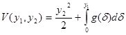
Clearly V is positive definite and satisfies an infinitesimal upper bound; moreover, V*(t, y₁, y₂) is negative definite. Thus it satisfies the theorem above.


Example 2: Consider the system

(*)

Where are as example 1 above and where are real continuous functions defined on the region {(t,y₁,y₂): 0t<, 0y₁²+y₂²r²} for some constant r>0 that satisfy

=0 (i=1, 2) (**)

This condition implies that g_i(t,0,0) =0 (i=1,2); thus y_i=0 is critical point and we wish to establish its asymptotic stability.

To establish asymptotic stability consider the same V function as before. However, with respect to the system (*) we now obtain V*(t,y_1,y₂) -2[(y₁²+y₂²)+y₁ g₁(t,y_1,y₂)+ y₂ g₂(t,y_1,y₂) using (**) given any there exists a number such that

for (j=1, 2)

|y₁ g₁(t, y1,y2)+ y₂ g₂(t,y_1,y₂)| for

Since | (i=1, 2) we obtain V*(t,y_1,y₂) -2(y₁²+y₂²)+4(y₁²+y₂²) provided y₁²+y₂^2.

Choose (any number less than will do) and determining the corresponding we obtain

V*(t,y_1,y₂) -(y₁²+y₂²), ()

Thus V* is negative definite on the set {{(t, y₁, y₂)| t, y₁²+y₂²²} and this shows that theorem 1 yields the desired result.

Consider the scalar equation (i),

where , where is a constant. We may think of as a damping term of a linear oscillator. It can be shown that if is also bounded above, and then every solution of the equation (i) together with its derivative approaches zero. This, however, does not follow from theorem 1. For consider the equivalent system



and the positive definite scalar function having an infinitesimal upper bound. However .

Thus is positive, but not negative definite.

For the problem such as the one consider on equation (i) above, it is natural to inquire whether the results and techniques discussed in chapter 2 for autonomous systems can be carried over to the nonautonomous cases. One difficulty in doing this is that the notion of invariant set, natural for autonomous systems, cannot be defined directly for non autonomous systems. However, for a class of problems that may be called asymptotically autonomous systems, analogous results do hold and we state one such theorem below.

Let f(t,y) and h(y) be continuous together with their first derivatives with respect to the components of y in a set {(t,y)|0} where is some set in y-space.


Definition: The system

(3.2)

is said to be asymptotically autonomous on the set Ω if
a) and this convergence is uniform for y in closed bounded subsets of Ω.
b) For every and every there exists such that


Example: Consider the scalar equation



This equation is asymptotically autonomous on any closed bounded se is a constant. For:



Uniformly with respect to y in Ω



whenever


Theorem 2: Suppose the system (3.2) is asymptotically autonomous on some set Ω in y-space. Suppose whenever y lies in a closed bounded set Suppose there exists a nonnegative scalar functionsuch thatwhere Ω . Let M be the largest positively invariant subset of Ω with respect to the limiting autonomous system

(3.3)

Then every bonded solution of approaches M as In particular, if all solutions of (3.2) are bounded, then every solution of approaches M.

We will now establish the asymptotic stability (global) of the zero solution of the system considered in Example 2 above. In the notation of previous theorem 2 we have




So that and Ω = {(y₁,y₂)|y₂=0}, that is the y₁ axis. On this set Ω

(*)

is asymptotically autonomous and the corresponding limiting system is



which is obtained from (*) by putting y₂=0. In order to apply theorem 2 above we must assume



for but also for where k>0 is constant. This insures that |f(t,y)| is bounded whenever |y| is bounded.

We observe next that every solution of



exists on and is then for as long as it exists we have from example



Therefore,



Thus by a familiar argument exists on and is bounded.

To apply theorem 2 we need to obtain M, the largest invariant subset of Ω with respect to the system (**) since every solution of (**) has the from where c₁ and c₂ are arbitrary constants M is clearly the origin and this, by theorem 2, proves the result.

Summary

A region of asymptotic stability is a set of points surrounding a stable equilibrium point for which every system trajectory starting at a point in the set asymptotically takes to the equilibrium point. This seminar paper is to develop and validate computationally good methods of estimating regions of asymptotic stability of nonlinear systems and apply Lyapunov’s second method.

In general we can summarize the main points of this seminar paper as follows:

• Lyapunov’s second method used to determine stability of differential equation without explicitly integrating the nonlinear differential equation.
• It also determines asymptotic stability and estimate the region of asymptotic stability (RAS) of both autonomous and nonautonomous nonlinear systems.
• For this Lyapunov’s direct method is very useful method for estimating the region of asymptotic stability for non linear system.

References

1. Ali Saberi, 1983. Stability and control of nonlinear singularly perturbed system, with application to high –gain feedback. Ph.D dissertation Michigan State University. East Lansing. FIND ONLINE

2. Fred Brauer and John A.Nohel, 1869. The Qualitative Theory of Ordinary Differential Equations. University of Wisconsin, over publication, Inc., New York. FIND ONLINE

3. Garrett Birkhoff Gion Carlorot,  Ordinary Differential Equations, 4th edition, John Wiley & Sons.FIND ONLINE

4. R. M. Murray, Z. Li and S. S. Sastri. Lyapunov stability theory. Caltech. FIND ONLINE

5. Mao, J. (1999) Differential Equation Stochastic. LaSalle theorems for SDEs, limits sets of SDEs.

6. Richard E.Williamson, 1997. Introduction to Differential Equations and Dynamical systems. the McGraw-Gill companies, Higher Education 20INB001, Dartmouth College. FIND ONLINE

7. G.P. Szegö, A contribution to Liapunov's second method: Nonlinear autonomous systems. Trans. ASME Ser. D.J.Basic Engrg., 84 (1962), 571-578.

Cite this paper

APA

Yadeta, Z. (2013). Lyapunov’s Second Method for Estimating Region of Asymptotic Stability. Open Science Repository Mathematics, Online(open-access), e70081944. doi:10.7392/Mathematics.70081944

MLA

Yadeta, Zelalem. “Lyapunov’s Second Method for Estimating Region of Asymptotic Stability.” Open Science Repository Mathematics Online.open-access (2013): e70081944.

Chicago

Yadeta, Zelalem. “Lyapunov’s Second Method for Estimating Region of Asymptotic Stability.” Open Science Repository Mathematics Online, no. open-access (March 20, 2013): e70081944. http://www.open-science-repository.com/lyapunovs-second-method-for-estimating-region-of-asymptotic-stability.html.

Harvard

Yadeta, Z., 2013. Lyapunov’s Second Method for Estimating Region of Asymptotic Stability. Open Science Repository Mathematics, Online(open-access), p.e70081944. Available at: http://www.open-science-repository.com/lyapunovs-second-method-for-estimating-region-of-asymptotic-stability.html.

Science

1. Z. Yadeta, Lyapunov’s Second Method for Estimating Region of Asymptotic Stability, Open Science Repository Mathematics Online, e70081944 (2013).

Nature

1. Yadeta, Z. Lyapunov’s Second Method for Estimating Region of Asymptotic Stability. Open Science Repository Mathematics Online, e70081944 (2013).

doi

Research registered in the DOI resolution system as: 10.7392/Mathematics.70081944.

This work is licensed under a Creative Commons Attribution 3.0 Unported License.